OK, this is a bit off-topic, but I was asked to write a short tutorial about how to make the flow map that I posted on Twitter. Why did I actually make it? Usually I am interested in faults and earthquakes, but sometimes secondary earthquake effects such as landslides can help us to find out about seismic activity. Since my next project will be about the Alps, I am currently looking a bit into landslides, too. The map shows a large landslide close to Jena, the Dohlenstein. This slide was activated several times in the past 300 years or so, but now seems to be stable. Behind the head scarp there is a small depression. I was wondering if this is perhaps just (paleo-)drainage, or if it could be the first hint for a new sliding plane and a larger future landslide. That’s why I made the flow map – if the depression has no outflow, it’s more likely to be related to newly forming tension cracks.
What do you need?
If you want to reproduce the map, you first need to install the free QGIS software. Download the standalone version here: https://www.qgis.org/en/site/forusers/download.html
Now we need the high-resolution topography data. Great news: 1 m LiDAR digital elevation models (DEMs) are available for entire Thuringia for free! Visit this website and navigate to Kahla.
Data download
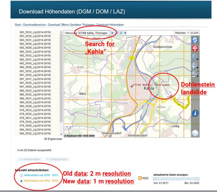
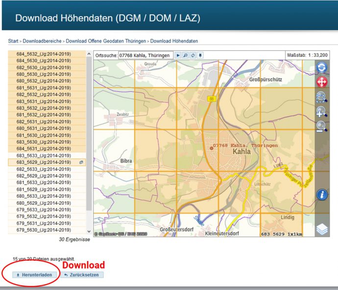
Select the latest data at the bottom left and simply click on the tiles that you want. Now you can download them (up to 20 files at once) as a zip-file. Choose the “DGM” option for download. DGM = digital terrain model (without trees and houses), DOM = digital surface model (with trees and houses). Unzip the folder. Now unzip all single files. You can delete the zip files now, and you should see *.XYZ and *.meta files for each tile.
Preparing the DEM
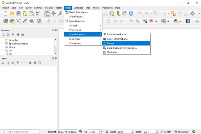
Now we want to combine the single tiles into a single DEM. Open QGIS, start a new project and choose “Raster” –> “Miscellaneous” –> “Merge”.
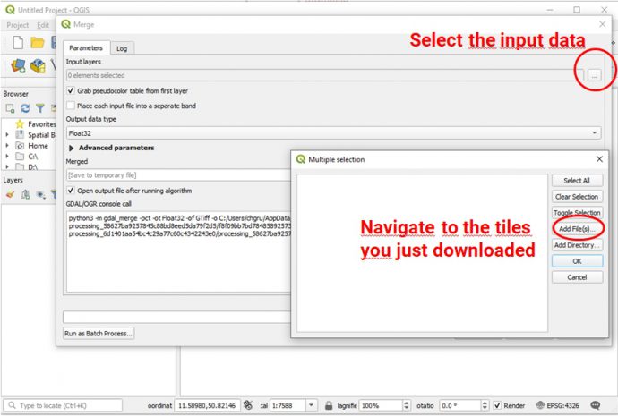
Find the XYZ-tiles that you have downloaded, define a name for the output file, check “Grab pseudocolour table from the first layer”, and click “run”, then “close”.
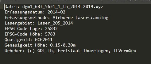
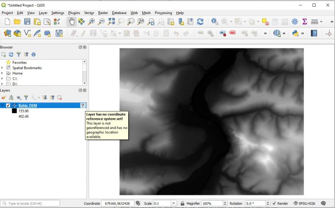
Now you should be able to see the data in QGIS. If you open one of the *.meta-files with a text editor, you can see the information on projection etc. The DEM comes in EPSG 25832, that’s ETRS89 / UTM Zone 32 North.
Click on the small question mark next to the DEM layer in the layer panel and choose EPSG 25832. Click OK. If you can’t see the DEM anymore, right-click on the layer and select “zoom to layer”.
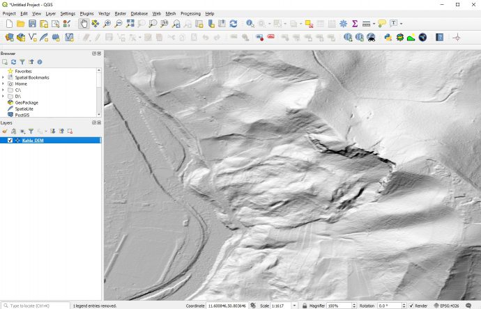
Right-click on the layer, select “Properties”, and choose “Hillshade” in the “render type” pulldown menu. Hit “apply” and magic happens. You can play around with the sun angle and the z-factor. Think of the latter as a vertical exaggeration. Since our data is in UTM, both the x-y-units and the z-units are in metres. Therefore, the z-factor is 1. If we had data with degrees as x-y-units, we would have to enter a conversion factor here, something like 0.00001 or so depending on the latitude. Check out the beautiful Dohlenstein landslide now:
Calculating the flow map
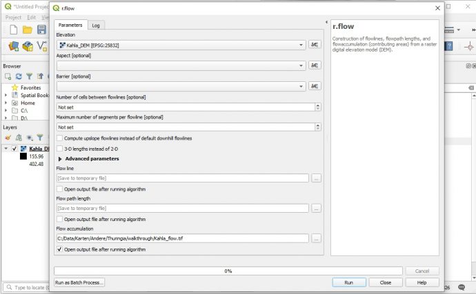
Now we want to calculate the flow map. From the menu, select “processing” –> “Toolbox”. A new side panel will open with lots of tools. Search for r.flow or find it in the GRASS toolbox.
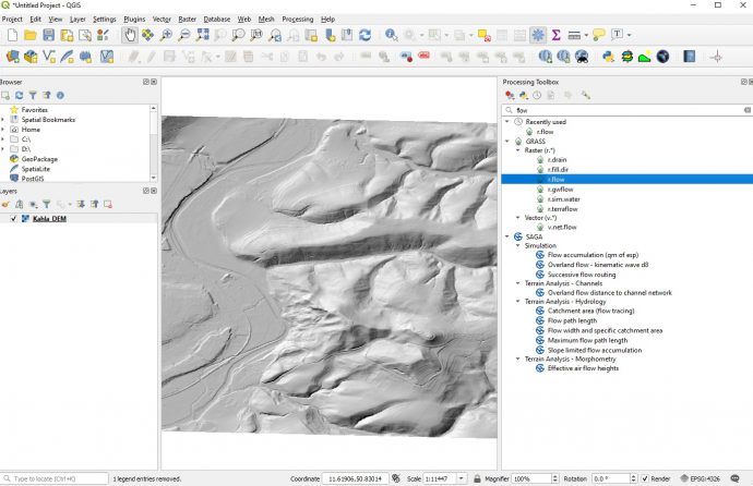
Make sure to use your DEM as an input file. Leave aspect and barrier file blank. Select an output filename and location. I leave all the other parameters in their default settings, you can play around with them of course.
After a few seconds or minutes, your flow map is calculated and displayed:
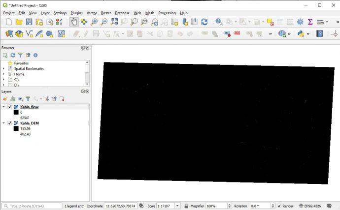
How disappointing! We need to make it a bit more beautiful, eh?
Making the map beautiful
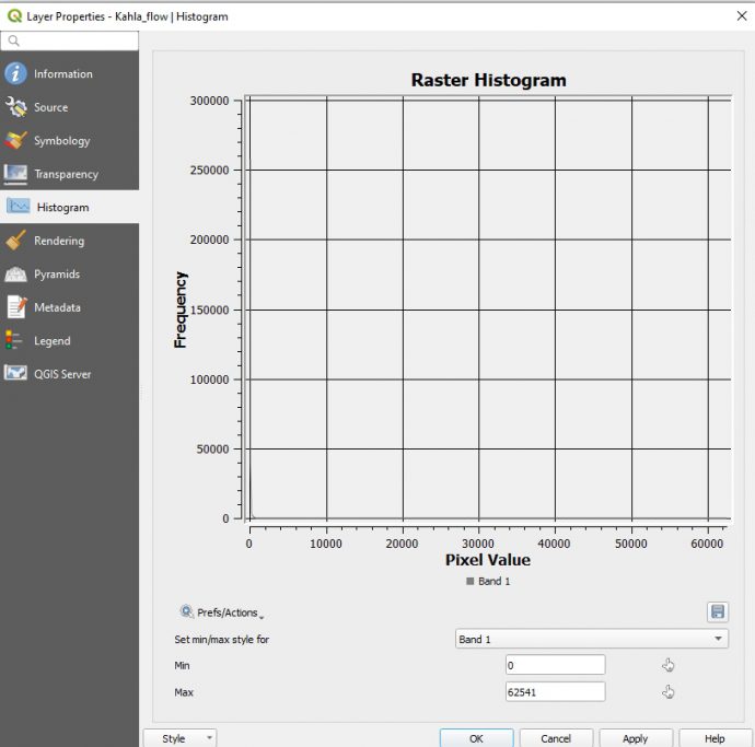
The biggest problem here is the colour code, of course. Right-click on the new layer, in my example “Kahla_flow”, select “Properties” and find the “Histogram” option. Click “compute histogram”. What we see is that the vast majority of values is below 1000. That’s why the colour scale is completely off.
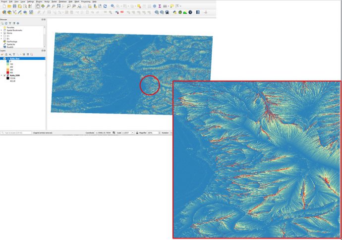
Now select “Symbology” and the render type: “singleband pseudocolour”. I use the colour ramp “spectral” and a range of 0-400 (found by looking at the histogram) with 5 classes. If you can’t see “spectral”, click the small triangle next to the colour ramp symbol and choose “all colour ramps”. This is also where you can invert the colour ramp, so that blue = low values:
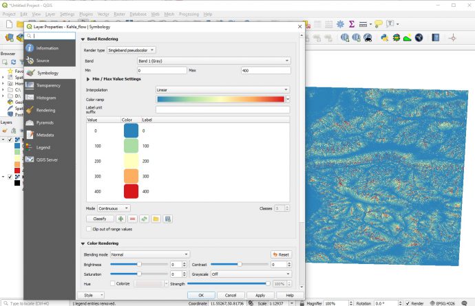
Now we’re getting close and it becomes clear what the flow algorithm actually does: Imagine you let it rain on your map and you look at the surface run-off. Red colours indicate cells where a lot of water passes through. That’s it. Let’s zoom into our landslide.
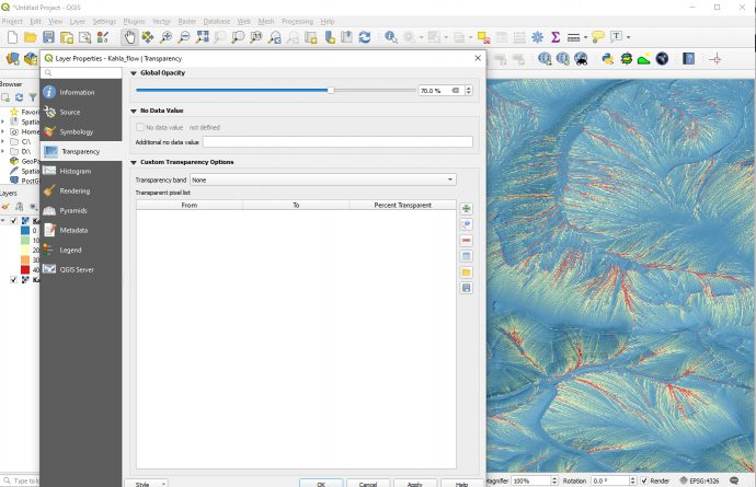
Still not very beautiful. Let’s give this layer a transparency. Right-click on the layer, select properties, find the “Transparency” settings and choose a value of 70%.
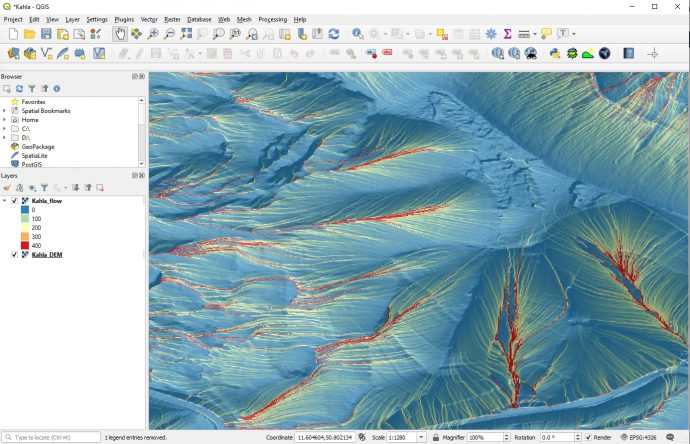
Almost there! In order to enhance the topogrpahy, I went back to the DEM and set the z-value to 5. Now the background hillshade is a bit more aggressive, which gives the whole scene a more dramatic appearance. That’s it, now you have the figure you wanted:
If you want to change the density of the flow lines, play around with the parameters of the flow algorithm. Another tip: If you see square artefacts in the hillshade, you can get rid of them in the “Properties” –> “Symbology” –>”Resampling” settings. Choose “bilinear” or “cubic” and “average” instead of “nearest neighbour”.
More info on the Dohlenstein
The horizontal bands that you can see in the DEM are partly agricultural terraces (for apple and plum trees), but mainly the Triassic layers that make up the bedrock. Actually, the Dohlenstein sits in an inverted graben that strikes ~NW-SE. Here the Muschelkalk sank into the underlying Buntsandstein. Later the whole area was uplifted and underwent erosion. The Buntsandstein is easier to erode than the Muschelkalk, so that now the Muschelkalk sticks out and forms a topographic high, although it’s a graben and not a horst. We see that quite a lot in Thuringia.
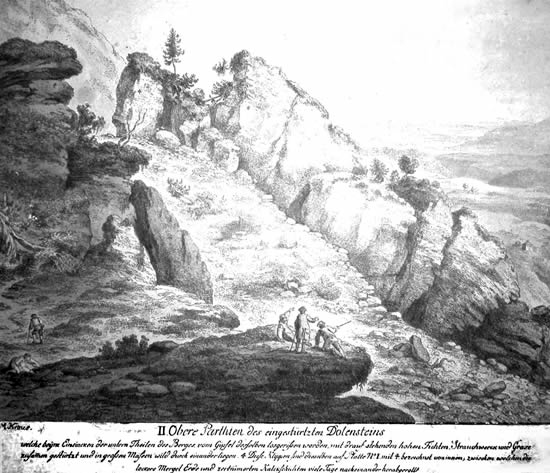
The first report of a landslide at the Dohlenstein is from 1740. Later reactivations happened in 1780, 1828, 1881, and 1920. When the main slide happened, the Saale River was blocked and partly dammed. Even today the river hasn’t managed to fully eroded the landslide body.
We made a little animation of the Dohlenstein landslide that we use for teaching in the Structural Geology group of FSU Jena:

By loading the video, you agree to YouTube’s privacy policy.
Learn more


No Comments
No comments yet.